
If you want to skip the story, go here. You will miss some embedded nuggets if you do. If you prefer the technical details, go here for the ExpandingExposures files: QMD, PDF, and HTML. The PDF is embedded at the end of the document.
The Quest Continues…
Antoni had just gotten back to the office. Vivian’s advice continued to rattle around his head. On the plane ride home, he read the paper she pointed out to him.
- It was an old paper, published in 1980, and seemingly unknown in the life insurance world even 75 years later.
- It derived an equivalence between Cox proportional hazards survival models and Poisson GLMs.
- Because of this, the exposure interval could be broken up whichever way you need to to reflect time-dependent changes in the data.
- For example, if new facts were observed about a case at a later time, the exposure could be divided at that point.
All of that justified (most of) what actuaries had been doing for eons. So nothing new, other than the comfort of being able to appeal to authority.
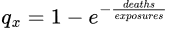
What it didn’t directly address was the exposure padding issue. As he settled into his chair and plugged in his neural link, he vaguely remembered an old identity relating hazards and mortality rates. The neural link sensed his thought pattern and immediately presented the background on the screen in front of him, starting with the relation:
But CyberLife’s experience studies relied on this approximation:

Were these close? The AI assistant prompted Antoni if he wanted it perform the calculation, but he declined. I don’t need AI to do everything, he thought, irritatedly. There was a growing movement for humans to do more of the thinking, and he was very much a partisan.
So he jotted down a quick derivation using power series and saw that the difference in the formulas was no worse than:
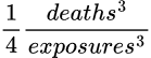
For this difference to be meaningful, the termination rates would have to have been a large fraction of exposures. This meant that the difference was only meaningful at the oldest ages for deaths. For the younger ages of the CyberTerm product, it may not be to be detectable for mortality. For lapses, though, it might be a different story.
So exact exposures could work, he thought happily, but with a twinge of anxiety. What about expected claims? The hazard-based formula could be inverted so that

I don’t think Grey will like this. His anxiety spiked. Yvette Grey was a well-respected, experienced actuary with very strong opinions and expertise on life insurance experience studies. She was adamant that things had to be done exactly her way. Antoni and Grey argued all the time about how to analyze the data. This will be no exception.

Excited and nervous, he got to work on rebuilding the experience study.
Designing a Study
Antoni is an expert in databases, database programming, and how to construct experience studies. Ultimately, the design of an experience study looks something like this:
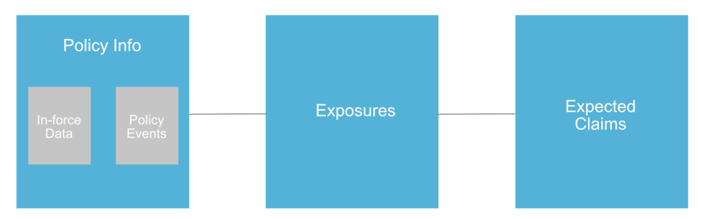
More concretely, you start with a policy in-force and event data, which may be combined in one table for life insurance:
| Policy Number | Issue Date | Termination Date | Facts |
| 1 | 3/3/2051 | 3/15/2051 | … |
| 2 | 7/14/2043 | NA | … |
| ⋮ | ⋮ | ⋮ | ⋱ |
Then you expand this into an exposures table:
| Exposure ID | Policy Number | Exposure Start | Exposure End | Time-Varying Facts |
| 1 | 1 | 3/3/2051 | 3/15/2051 | … |
| 2 | 2 | 7/14/2043 | 12/31/2043 | … |
| 3 | 2 | 1/1/2044 | 7/13/2044 | … |
| 4 | 2 | 7/14/2044 | 12/31/2044 | … |
| ⋮ | ⋮ | ⋮ | ⋮ | ⋱ |
In words, this can be done as follows:
- Form a timeline of policy anniversaries (or monthly or quarterly “mode-aversaries”) which represent the ending dates of the exposure periods. In the example above for policy 2, this corresponds to July 13, the day before the anniversary of the issue date. For policy 1, this is the death date.
- Form another timeline representing the calendar year breaks aligned to your study window. In the example above, these are the year-end days, December 31.
- Either cross join the timelines with the policy census and merge the two lists, or merge the two timelines and cross join with the census. Sort as needed.
- The starting date for the exposure will be the day after the end of the previous period, except when there is no previous period. In this case, use either the issue date or the study start date as appropriate.
The rest is basically data engineering, and serious data engineering at that. For example, a large company might have millions of policies. Expanding the exposures out like this will result in tens of millions to hundreds of millions of exposure records depending on how wide the study window is and how fine the company wants to subdivide the timeline. For example, in health, calendar month granularity is common. This situation demands careful planning and forethought. You will need to consult with your data architects for optimal design, implementation, and management.

An Aside About This Image
I asked DALL-E for the following to illustrate an actuary laboring heavily: imagine a scene of an ancient Egyptian hauling one of the pyramid stones, but the ancient Egyptian has been replaced by an actuary.
Not only did it provide the image above, but it gave some color commentary as follows:
Certainly! Let me conjure an image that blends the ancient and the modern. Imagine an actuary, dressed in a crisp suit, standing amidst the sun-baked sands of ancient Egypt. His pocket protector bulges with pens, and his calculator is ever at the ready. But instead of a whip-wielding pharaoh overseeing the construction, it’s the stern gaze of an auditor that weighs upon him. The massive stone he hauls is no ordinary pyramid block; it’s a cubic monolith, etched with financial equations and risk assessments. The actuary’s brow furrows as he calculates the optimal angle for dragging this burden across the desert. The sun beats down mercilessly, and the hieroglyphs on the stone seem to mock him. Yet, with unwavering determination, he pulls forward, inch by inch, dragging the weight of probabilities and mortality rates toward the pinnacle of financial stability. And so, in this surreal fusion of epochs, the actuary becomes a modern-day pyramid builder, constructing not tombs for pharaohs but financial models for the ages. 🌟🔍📊
Tooling
While this can all be done in R and Python, any serious study will be done using tools which can handle large volumes of data efficiently.
- DIY in Excel: PowerQuery can probably handle it, but compared to other tools, it is terribly inefficient.
- DIY in R and Python: R (and soon Python) can be engineered to carry this out on even some fairly large portfolios, and the accompanying example does so in R. Because of downstream storage and reporting needs, it is probably not the best option.
- Pre-built libraries: Matt Heaphy has written packages in R and Python which do an excellent job of building out the exposure base. Whether it makes sense to use depends on your context.
- Databases: SQL databases readily optimize for parallelism, and the pipelines can be built and maintained by non-actuaries. Given the potential size of an experience study system, you will likely go this route for an in-house solution at some point.
- Pre-built systems: Insight Decision Solutions is one among several vendors who provide experience studies systems. I mention them because I have worked with that system before. This approach is often easier for the typical actuary to live with long-term than in-house systems.
Much goes into tooling decisions, such as ease of use, cost, maintainability, auditability, performance, and interoperability.
Design Considerations
If you were to develop your own system, there are several design considerations for build and maintenance.
Incremental Builds
With one exception, exposures don’t change once they are calculated. It is fact of the past. It is possible to set up the build process so that only the incremental calendar period is added to the table, such as the latest month, quarter, or year of interest.
Maintaining the Exposure Table
It is reality that a company is only on the risk for well-defined times, between the issue date and the termination date. Thus, the exposure for a given calendar period should be created once, right?
Yes and no.
Yes, because for the majority of the situations, this is the case, but…
If you keep the study relatively current, late reported terminations might force a recalculation of exposures. It is potentially expensive to rebuild the exposures every calendar period, plus rebuilding exposures creates headaches for reproducibility of prior work. Archiving numerous very large tables gets cumbersome and expensive.
One approach is to create negative exposure records which “undo” the exposures you intend to back out and then add an “as-of” date to the exposures table so that one can recreate the exposures at a given point in time. The value here is that only one table ever need to be built, maintained, and backed up. Insurance is transactional, and experience studies can be transactional too.
Maintaining Expected Claims Tables
Studies usually have some additional information on what the expected claims should be. This is calculated for each row of the exposures table.
Expected claims information is volatile and should be kept separate from the exposures. There are also often numerous bases for different purposes, such as industry tables, industry tables with factors, and custom internal assumptions. These can also differ by event type, such as mortality, lapse, and exercise of other options.
I cannot recommend a “best” data engineering approach, although I would probably choose a hybrid of the following:
- Put all of the expected bases into a single table in long format. Managing the schema is easier, but the tables become large and difficult for reporting systems to query efficiently.
- Pull all of the expected bases into a single table, with a separate column for each table. This makes querying faster, yet the downside is that adding and removing columns can make data engineering complicated.
- Use separate tables for each basis.
What works best for you will depend on how big your study is and how many and how complex the claims bases are. If I had to choose, I would put “eternal” bases like industry tables in the first or second type, and put “ephemeral” bases like LDTI and IFRS assumptions in separate tables.
Dealing with Incurred Claims
Claims can be volatile over time. Claims may not be reported in a timely fashion, and complicated claims may be subject to lengthy investigation or litigation delays. Moreover, events in life insurance tend to be rare. Thus, claims should be held separate from the exposure tables, potentially with special handling for claims incurred but not yet reported. This means your IBNR processes should be engineered to help complete the experience study picture.
Other Event Types
Experience studies can cover a broad range of events. The study should be designed to reflect the underlying behavior accurately. It comes down to whether the event terminates the exposure.
If the event terminates the exposure like mortality and lapse, then we do as we have here. We would also want to consider the ratios of events to exposures to be a cumulative hazard and model accordingly.
However, if the event doesn’t terminate the exposure, like a medical claim, then the ratio is just a regular rate that may or may not be a probability. Poisson models are still valid, and no transformations are necessary as in the terminating case. Medical claims also allow for different modeling types than what is considered here, so consider your needs accordingly.
There is another wrinkle with respect to mortality and lapse. Mortality can happen at any time, but some kinds of lapse can only occur on a premium due date. For mortality, that means we spread the exposure out uniformly, as we do here. However, for lapse, that implies we must concentrate the exposure at the premium due date (really the day before).
Why is this so? Imagine I have a collection of policies with annual due dates, but I am only looking at experience in a particular quarter or month, say March. If I modeled the exposure uniformly, then exposures for policies which cannot lapse in March get included in the denominator. This suppresses the measures accordingly.
For Next Time
- Antoni has a showdown with Grey (because drama).
- I provide a concrete, easy example of why the old approximation might distort estimation of old age mortality.

Leave a comment