The Machine Learning Company

Synthetic Data, From Scratch

When I decided I would make a series on how to build experience studies, I discovered a sad fact. There are no publicly available life insurance datasets, or if they are out there, they are perhaps out of sight in the deep or dark web. Rather than flirt with felons, I thought it far better to just make a dataset up based on my experiences.

This post will cover the high-level features and my experiences, including such exciting topics as:

• Creating a slate of preferred characteristics with the dependency structure I wanted using vine copulas (the only math-heavy bit of this post)
• The joys and woes of reproducible parallel simulation in R
• Why Python might not be a great choice for this sort of thing (for now)

If you want to see the technical details, there is a Quarto document waiting for you at the bottom of this blog. The Github repo is also available here.

The Setting

The story I started with the last post was that an analyst was going to analyze experience on a block of policies where the experience is deteriorating. The analyst has to find out why. It happens to be set in the future, where humans can now opt to hybridize with robots. The life insurance market is similar but not the same for these risks, and it is a new line of business with new issues. For example, preferred criteria in this (simplified) example are the Bot Mass Index (BMI), oil pressure, and oil viscosity. The similarities to Body Mass Index (BMI), blood pressure, and cholesterol are not all that coincidental.

Getting Started

I have the Individual Life Experience Committee dataset handy, so I pulled a tally of exposures based on Term business in duration 1, ages 18 to 70, issued under a four-class preferred system. This included information on face amount bands.

To reflect a growing portfolio, I replicated the tally across issue years 2041 to 2054, where the early years have a lower proportion and the later years have a higher proportion.

From there, I simulated what day of the year the policy was issued. Based on my experience, policies tend to issue more toward the end of the year than the beginning. This is due to sales and marketing incentives skewing production to the end of the year at the expense of the following quarter.

I did simulate some face amounts for completeness, but they aren’t that important in this analysis. The only thing that matters is that there are differences in the “low face” and “high face” groups when it comes to mortality and lapse outcomes.

Inventing Risk Factors

In this brave new world, the human-robot hybrids now have a different risk profile. Even though these hybrids probably won’t use hydraulics if they ever do come into existence, I imagined that they still rely on oil for their mechanical functions. Oil pressure and oil viscosity now influence mortality, as does build.

It is easy to create distributions for a single risk factor. What is not so easy is modeling their interdependence. In the real world, it is rare that characteristics involving health are independent. For example, cholesterol and blood pressure tend to increase with BMI.

Here is what a naive analyst might do:

• Modeling the distributions separately and then multiplying them together as if they are independent, which is going to be wrong.
• Modeling them with a multivariable parametric distribution might work, but which one? And how do you deal with the curse of dimensionality?

Why do I know that a naive analyst would do this? Maybe I was naive once. Maybe.

The Wonderful World of Vine Copulas

When I first had to deal with modeling joint distributions of preferred criteria, I was drawn to copulas. At the time, the best available was Roger Nelson’s An Introduction to Copulas. It is the classic text on the subject.

Sklar’s Theorem

There is a remarkable theorem about probability distributions called Sklar’s Theorem. It states that every multivariable cumulative distribution function can be rewritten as a function of its marginal CDFs. This function, called the copula, is a probability distribution in its own right on the unit hypercube.

Consequences include:

• You can understand the dependencies between random variables separately from the marginal univariate distributions of the random variables.
• You can mix and match copulas and marginal distributions. Perhaps combine a t copula with gamma, normal, and Poisson marginals.
• It can also be shown that any probability distribution can be decomposed using bivariate copulas, although the final form is a bit messy as we will see.

If you are in the data modeling business, the next obvious question to ask after reading Nelson’s book is how can you model data with it. At the time, the answer was sadly “not well”.

Awash in (Bivariate) Copulas

There is a long list of bivariate copulas, such as the normal, t, Gumbel, Clayton, Frank, BBx series, and Joe copulas.

There are, however, very few copulas of higher dimension. Off the top of my head, only the normal and t copulas allow for higher dimensional modeling natively. To add insult, only the Archimedean copulas are composable in a way that lets you build up a more complicated copula from simpler copulas.

Thus, copula modeling was limited to bivariate or special cases.

It is only more recently that research into vine copulas has matured sufficiently to allow data modelers to flexibly model higher dimensional datasets using copulas.

The Vine Copula

A small but productive group of researchers have worked on the problem of vine copulas. Vine copulas start with the idea that any probability distribution can be decomposed using bivariate copulas as can be done in the following for a three-variable density:

This derivation is taken from Claudia Czado’s Analyzing Dependent Data with Vine Copulas, pp. 77-78.

The complicating item here is the first copula density

This function will in general depend on the conditioning variables, rendering the problem of using this decomposition to build up a copula difficult. However, the simplifying assumption of vine copulas is to drop that dependency and fit a copula without direct dependence on other variables.

Freed of that constraint, you can now successively build up dependency structures on a dataset as follows:

• For each variable, if necessary, replace the variable with its transform to the uniform distribution. See the probability integral transform for more info. This replaces the x_i with u_i.
• Compute pairwise measures of association between these variables, typically using Kendall’s Tau.
• Using these measures, build a graph of dependencies between the variables meeting certain conditions, namely that the graph forms a tree (no loops).
• Each point represents a variable with associated data on the uniform scale, and each edge represents the dependency relationship.
• For each edge in the graph, find a bivariate C(u_i,u_j) copula which best fits the associated pair of data vectors.
• Applying the fitted copula to the associated data now creates a new vector of data on that edge. For example, u₁₂=C₁₂(u₁,u₂) is a new vector of data for the edge connecting u₁ and u₂.
• Each edge now has a vector of (uniformly distributed) data, and there is one less column than before.
• Apply the procedure on this derived data
• Continue until there are no more pairs of data to model.

Thankfully, there are mature libraries that you can use to do this in R (rvinecopulib) and Python (pyvinecopulib).

And that’s all the hard math in this post! If you are craving more math, I recommend these two books.

	Analyzing Dependent Data with Vine Copulas: A Practical Guide With R, by Claudia Czado Amazon | Springer | Barnes & Noble
	Dependence Modeling with Copulas, by Harry Joe Amazon | Taylor & Francis

The Preferred Risk Distribution

That machinery helped me build the following distribution:

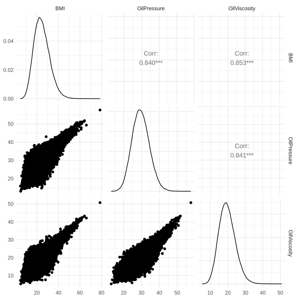
I wanted a lot of dependency between characteristics, and candidly, I may have gotten a little carried away with the dependencies. However, it ended up getting the upper tail dependency that I was looking for.

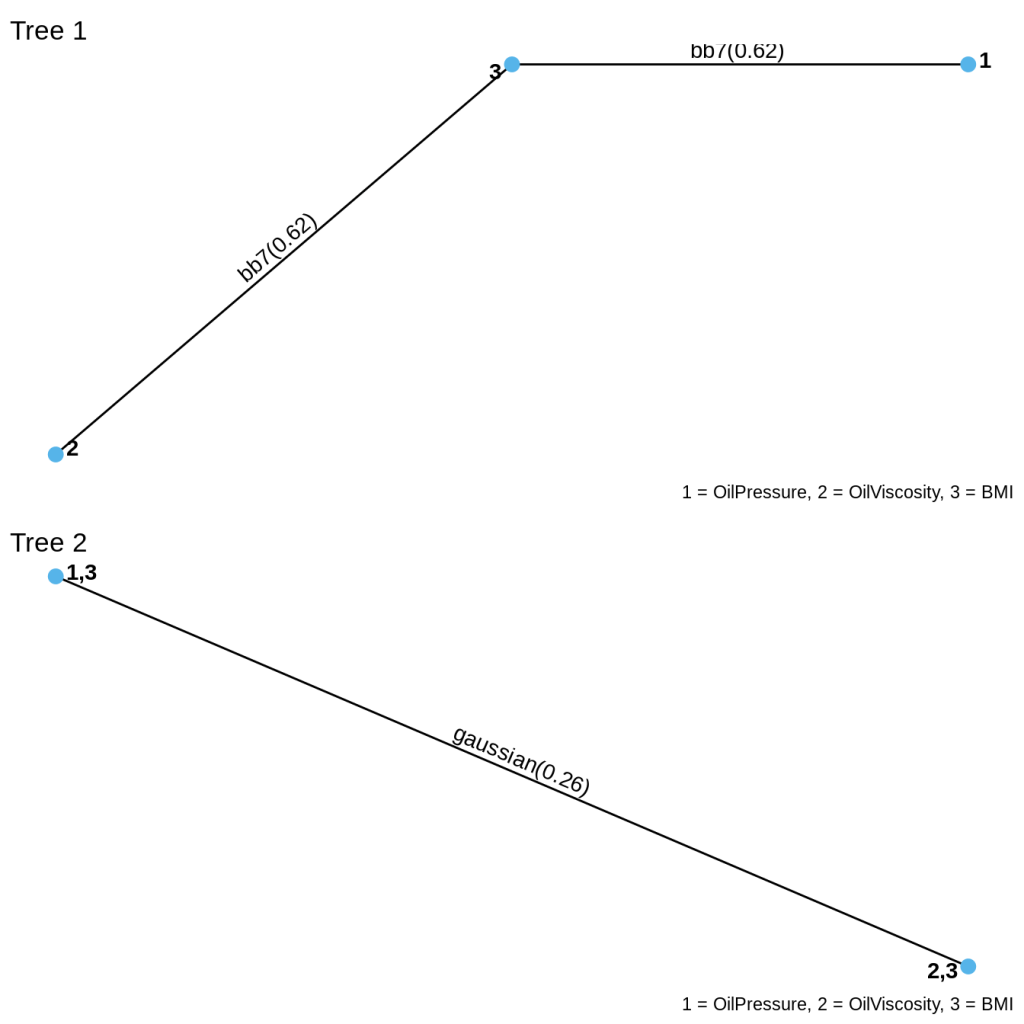
Here is the vine structure. You can see that at the first level, BMI depends on viscosity and on pressure via BB7 copulas. The second level of dependency is Gaussian and says that pressure and viscosity, given BMI, has Gaussian dependence.

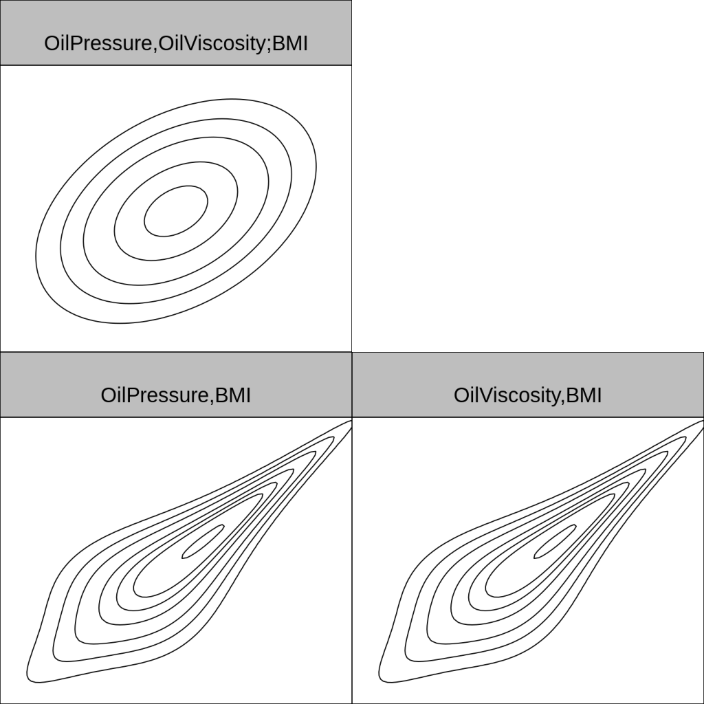
Here is what the copulas themselves look like, using normal margins.

Parallelism in R

With frequent practice, you become a power user in any software package (or really anything, like sports, art, your job, etc.) You can see in my R code the result of years of practice working with data and the workhorse packages I use, such as data.table, the tidyverse, ggplot2, and so on.

I want to touch on two major components of the R code and how they work together. Parallelism and simulation.

R makes parallelism very easy. If you can design your code to accommodate R’s parallelism, then R will take care of many of the details.

Simulation can be done in parallel, but with a catch. You have to use a special random number generator to ensure that the computations are reproducible. You can see this at the top of the Quarto document with my reference to the L’Ecuyer-CRMG generator. Not doing so will cause significant problems, such as inconsistent and erroneous results in my case.

I used parallel simulation to simulate the mortality and lapse outcomes for each policy. The performance gains are significant. With 16 cores, simulation takes about 12 minutes. Without parallelism, this takes hours.

Why should you design for parallelism from the beginning? It’s all about time efficiency. It is rare that code works right the first time. There were numerous bugs in the simulation code that needed to be worked out, and minutes versus hours between iterations makes a huge difference.

Unfortunately, the Python world is still catching up.

R vs Python: R Wins?

I wanted to redo what I did in R in Python for a few reasons:

• Exercise my Python skills
• Get acquainted with Polars
• Appeal to a broad audience

You can see in the Jupyter notebook that in many ways, the R and Python implementations are pretty close, with perhaps one glaring exception.

Impaired Parallelism

Python has a design limitation which makes parallelism difficult. In the early days of Python development, the designers put in something called the Global Interpreter Lock (GIL). The GIL only allows one thread to control the Python interpreter at any given time. Global locks ensure safe memory access, but they can degrade performance and prevent parallelism from functioning the way you might want.

In Python’s case, the GIL guarantees that only one thread of execution can use the interpreter at any given time. Thus, if I try to run a custom Python function in parallel (perhaps via lambda), all the threads have to wait their turn on the GIL to execute the custom Python function. As far as I can tell, I would have to write a custom C function in order to break through this bottleneck. I decided that was too much for this project.

On the bright side, the Python community plans to make the GIL optional in version 3.13.

Parallel Random Number Generation in Python

I found myself concerned about the advice I was getting online about how to reproducibly generate random numbers in parallel in numpy. If you use search or use an LLM, you will get advice which might lead you down a path where the random numbers might overlap, creating hidden dependencies in your simulation. For example, one approach suggested that I create a random number generators for each thread, and then seed them using a random sequence from the originating function. I would be concerned that you will end up with overlapping sequences of random numbers. Perhaps my concerns are overblown.

In any event, the numpy authors have some advice on parallel random number generation. The tyranny of the GIL makes all of this moot for now.

Other Quirks of R and Python

Here are some other quirks that surfaced as I went.

In Python:

• Polars is verbose. Writing Polars syntax to create a column is remarkably convoluted. Object-oriented predicates? As a developer, I can see the allure; as a user, I would prefer the simplicity of tidy’s syntax.
• Pandas is getting better, but not yet as fast as Polars. Pandas is easier to use than Polars, though.

In R:

• Occasional name conflicts between libraries, a minor inconvenience
• There were a few semantic gotchas when calling functions when defining columns in data.table.

That said, were it not for the GIL issue, using either Python or R would have been roughly equivalent in terms of effort and outcomes.

What’s Next

If you want a sneak peak at the issues I have baked into the simulated policy census, including the assumptions I used, please feel free to have a look at the R or Python code.

The next post will turn to building an experience study, and our hero returns to help our innovative life insurer get back on track. One hopes his mood will improve.

The Quarto Document